Section 2 Baseline: Varying organism size

Here we show all of the data for the baseline experiment in which we vary organism size while all other parameters are set to their default values.

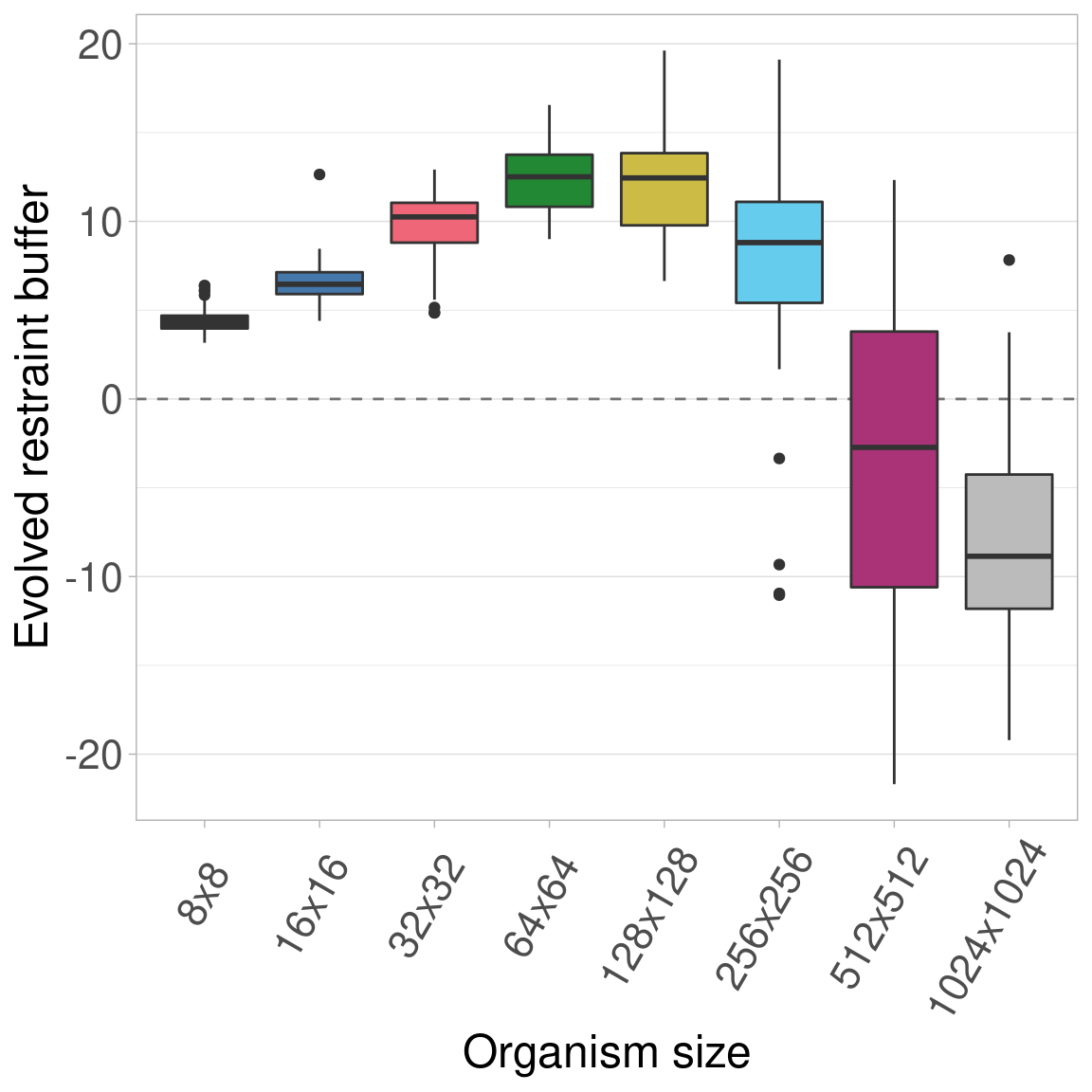
For this original experiment, we also tested size 8x8 and 1024x1024 organisms. In the paper, however, we only included sizes 16x16 to 512x512. Size 8x8 organisms are quick to run, but these smaller organisms see the most noise in the fitness data. Conversely, size 1024x1024 organisms take so long to run that it was not computationally feasible to run them for each experiment.

Here, we show these results for the baseline experiment, including these additional sizes. The configuration script and data for the experiment can be found under 2021_02_26__org_sizes/ in the experiments directory of the git repository.

2.1 Data cleaning

Load necessary R libraries

library(dplyr)
library(ggplot2)
library(ggridges)
library(scales)
library(khroma)

Load the data and trim to only include the final generation

# Load the data
df = read.csv('../experiments/2021_02_26__org_sizes/evolution/data/scraped_evolution_data.csv')
# Trim off NAs (artifacts of how we scraped the data) and trim to only have gen 10,000
df2 = df[!is.na(df$MCSIZE) & df$generation == 10000,]

Group and summarize the data to ensure all replicates are present.

# Group the data by size and summarize
data_grouped = dplyr::group_by(df2, MCSIZE)
data_summary = dplyr::summarize(data_grouped, mean_ones = mean(ave_ones), n = dplyr::n())

Clean the data and create a few helper variables to make plotting easier.

# Calculate restraint value (x - 60 because genome length is 100 here)
df2$restraint_value = df2$ave_ones - 60
# Make a nice, clean factor for size
df2$size_str = paste0(df2$MCSIZE, 'x', df2$MCSIZE)
df2$size_factor = factor(df2$size_str, levels = c('8x8', '16x16', '32x32', '64x64', '128x128', '256x256', '512x512', '1024x1024'))
df2$size_factor_reversed = factor(df2$size_str, levels = rev(c('8x8', '16x16', '32x32', '64x64', '128x128', '256x256', '512x512', '1024x1024')))
data_summary$size_str = paste0(data_summary$MCSIZE, 'x', data_summary$MCSIZE)
data_summary$size_factor = factor(data_summary$size_str, levels = c('8x8', '16x16', '32x32', '64x64', '128x128', '256x256', '512x512', '1024x1024'))
# Create a map of colors we'll use to plot the different organism sizes
color_vec = as.character(khroma::color('bright')(7))
color_map = c(
  '8x8' =       '#333333',
  '16x16' =     color_vec[1],
  '32x32' =     color_vec[2],
  '64x64' =     color_vec[3],
  '128x128' =   color_vec[4],
  '256x256' =   color_vec[5],
  '512x512' =   color_vec[6],
  '1024x1024' = color_vec[7]
)
# Set the sizes for text in plots
text_major_size = 18
text_minor_size = 16 

2.2 Data integrity check

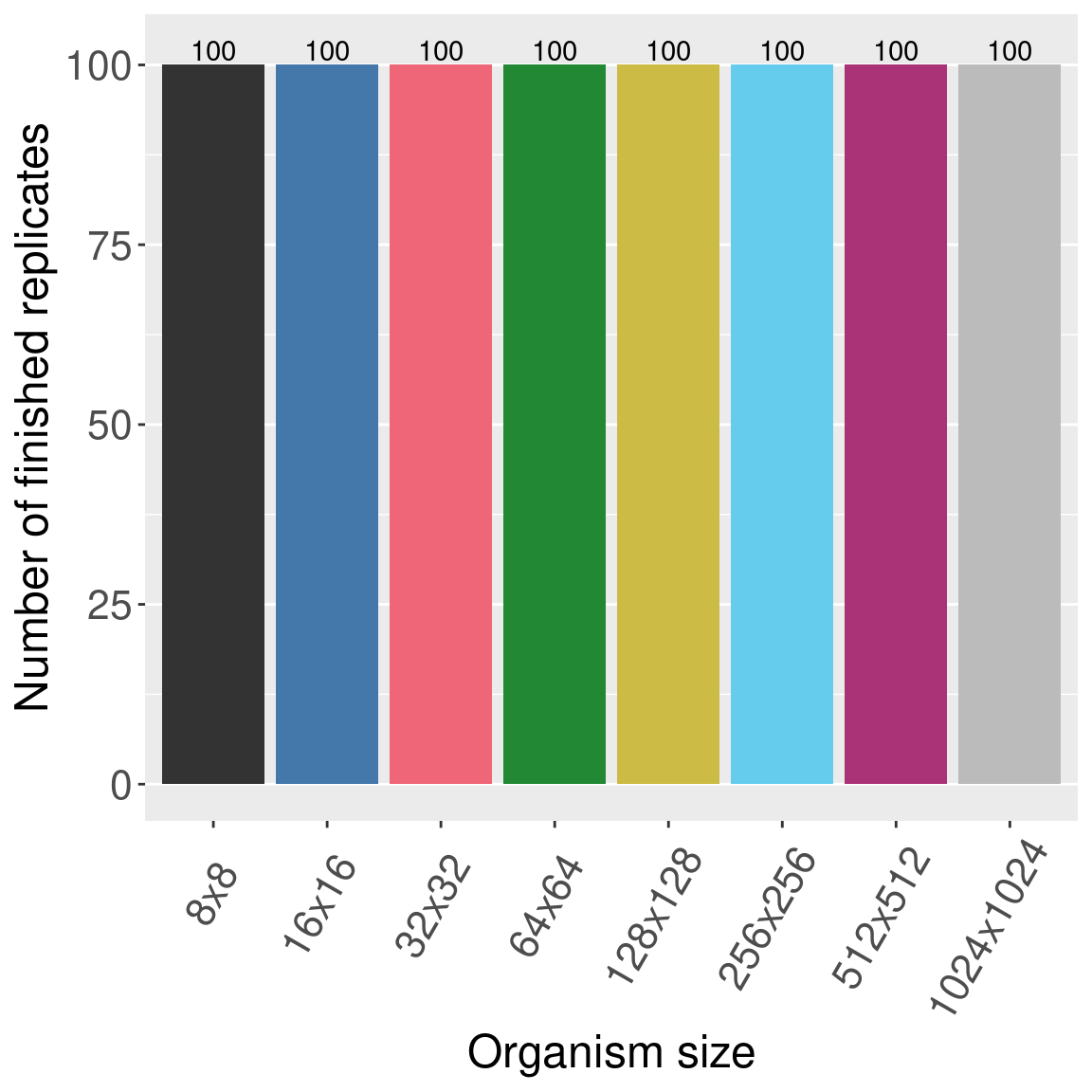
Now we plot the number of finished replicates for each treatment to make sure all data are present. Each bar/color shows a different organism size.

2.3 Aggregate plots

Here we plot all the data at once.

2.3.1 Boxplots

2.3.2 Raincloud plots

We can plot the same data via raincloud plots.

## Picking joint bandwidth of 1.16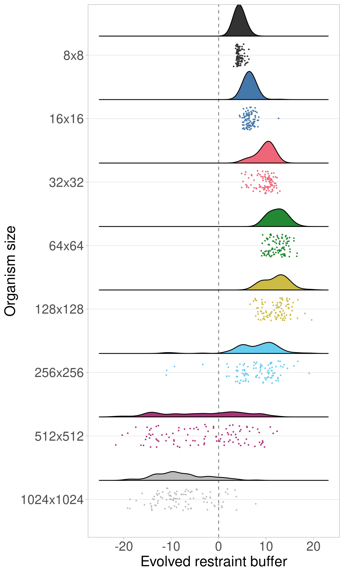

2.4 Statistics

First, we perform a Kruskal-Wallis test across all organism sizes to indicate if variance exists. If variance exists, we then perform a pairwise Wilcoxon Rank-Sum test to show which pairs of organism sizes significantly differ. Finally, we perform Bonferroni-Holm corrections for multiple comparisons.

  res = kruskal.test(df2$restraint_value ~ df2$MCSIZE, df2)
  df_kruskal = data.frame(data = matrix(nrow = 0, ncol = 3))
  colnames(df_kruskal) = c('p_value', 'chi_squared', 'df')
  df_kruskal[nrow(df_kruskal) + 1,] = c(res$p.value, as.numeric(res$statistic)[1], as.numeric(res$parameter)[1])
  df_kruskal$less_0.01 = df_kruskal$p_value < 0.01
  print(df_kruskal)

##         p_value chi_squared df less_0.01
## 1 1.506351e-127    610.2553  7      TRUE

We see that significant variation exists, so we perform pairwise Wilcoxon tests on each to see which pairs of sizes are significantly different.

size_vec = c(16, 32, 64, 128, 256, 512)
df_test = df2
df_wilcox = data.frame(data = matrix(nrow = 0, ncol = 5))
colnames(df_wilcox) = c('size_a', 'size_b', 'p_value_corrected', 'p_value_raw', 'W')
for(size_idx_a in 1:(length(size_vec) - 1)){
  size_a = size_vec[size_idx_a]
  for(size_idx_b in (size_idx_a + 1):length(size_vec)){
    size_b = size_vec[size_idx_b]
    res = wilcox.test(df_test[df_test$MCSIZE == size_a,]$restraint_value, df_test[df_test$MCSIZE == size_b,]$restraint_value, alternative = 'two.sided') 
    df_wilcox[nrow(df_wilcox) + 1,] = c(size_a, size_b, 0, res$p.value, as.numeric(res$statistic)[1])
  }
}
df_wilcox$p_value_corrected = p.adjust(df_wilcox$p_value_raw, method = 'holm')
df_wilcox$less_0.01 = df_wilcox$p_value_corrected < 0.01
print(df_wilcox)

##    size_a size_b p_value_corrected  p_value_raw      W less_0.01
## 1      16     32      4.406735e-21 4.406735e-22 1045.5      TRUE
## 2      16     64      1.790650e-32 1.193767e-33   51.5      TRUE
## 3      16    128      2.585339e-31 1.988723e-32  147.0      TRUE
## 4      16    256      1.864978e-03 6.216595e-04 3599.0      TRUE
## 5      16    512      3.596138e-17 4.495172e-18 8547.0      TRUE
## 6      32     64      2.103060e-15 3.004372e-16 1654.5      TRUE
## 7      32    128      1.857809e-09 4.644523e-10 2449.5      TRUE
## 8      32    256      8.472946e-03 4.236473e-03 6171.0      TRUE
## 9      32    512      1.338207e-26 1.216552e-27 9459.5      TRUE
## 10     64    128      4.429461e-01 4.429461e-01 5314.5     FALSE
## 11     64    256      2.515682e-15 4.192803e-16 8329.0      TRUE
## 12     64    512      1.552625e-31 1.109018e-32 9873.0      TRUE
## 13    128    256      4.763656e-12 9.527311e-13 7921.5      TRUE
## 14    128    512      3.610598e-30 3.008832e-31 9759.0      TRUE
## 15    256    512      7.155324e-19 7.950361e-20 8730.5      TRUE