Section 6 Population size experiment

By default, all populations contain 200 organisms. This experiment tested if increasing the population size to 2,000 organisms has any substantial effect on evolved restraint.

This experiment was initially conducted to find our default parameters. However, the data shown here were reran (with new random number seeds) when we decided to investigate population size in the paper.

The configuration script and data for the experiment can be found under 2021_03_06__pop_size/ in the experiments directory of the git repository.

6.1 Data cleaning

Load necessary libraries

library(dplyr)
library(ggplot2)
library(ggridges)
library(scales)
library(khroma)

Load the data and trim include only the final generation data for sizes 16x16 to 512x512.

# Load the data
df = read.csv('../experiments/2021_03_06__pop_size/evolution/data/scraped_evolution_data_200.csv')
df = rbind(df, read.csv('../experiments/2021_03_06__pop_size/evolution/data/scraped_evolution_data_2k.csv'))
# Trim off NAs (artifacts of how we scraped the data) and trim to only have gen 10,000
df2 = df[!is.na(df$MCSIZE) & df$generation == 10000,]
# Ignore data for size 8x8 and 1024x1024
df2 = df2[df2$MCSIZE != 8 & df2$MCSIZE != 1024,]

We group and summarize the data to ensure all replicates are present.

# Group the data by size and summarize
data_grouped = dplyr::group_by(df2, MCSIZE, POP)
data_summary = dplyr::summarize(data_grouped, mean_ones = mean(ave_ones), n = dplyr::n())

## `summarise()` has grouped output by 'MCSIZE'. You can override using the `.groups` argument.

We clean the data and create a few helper variables to make plotting easier.

# Calculate restraint value (x - 60 because genome length is 100 here)
df2$restraint_value = df2$ave_ones - 60
# Make a nice, clean factor for size
df2$size_str = paste0(df2$MCSIZE, 'x', df2$MCSIZE)
df2$size_factor = factor(df2$size_str, levels = c('16x16', '32x32', '64x64', '128x128', '256x256', '512x512', '1024x1024'))
df2$size_factor_reversed = factor(df2$size_str, levels = rev(c('16x16', '32x32', '64x64', '128x128', '256x256', '512x512', '1024x1024')))
data_summary$size_str = paste0(data_summary$MCSIZE, 'x', data_summary$MCSIZE)
data_summary$size_factor = factor(data_summary$size_str, levels = c('16x16', '32x32', '64x64', '128x128', '256x256', '512x512', '1024x1024'))
# Create a map of colors we'll use to plot the different organism sizes
color_vec = as.character(khroma::color('bright')(7))
color_map = c(
  '16x16' =     color_vec[1],
  '32x32' =     color_vec[2],
  '64x64' =     color_vec[3],
  '128x128' =   color_vec[4],
  '256x256' =   color_vec[5],
  '512x512' =   color_vec[6],
  '1024x1024' = color_vec[7]
)
# Set the sizes for text in plots
text_major_size = 18
text_minor_size = 16 

6.2 Data integrity check

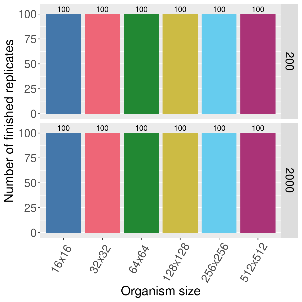
Now we plot the number of finished replicates for each treatment to make sure all data are present. Rows show the number of samples used for fitness. Each bar/color shows a different organism size.

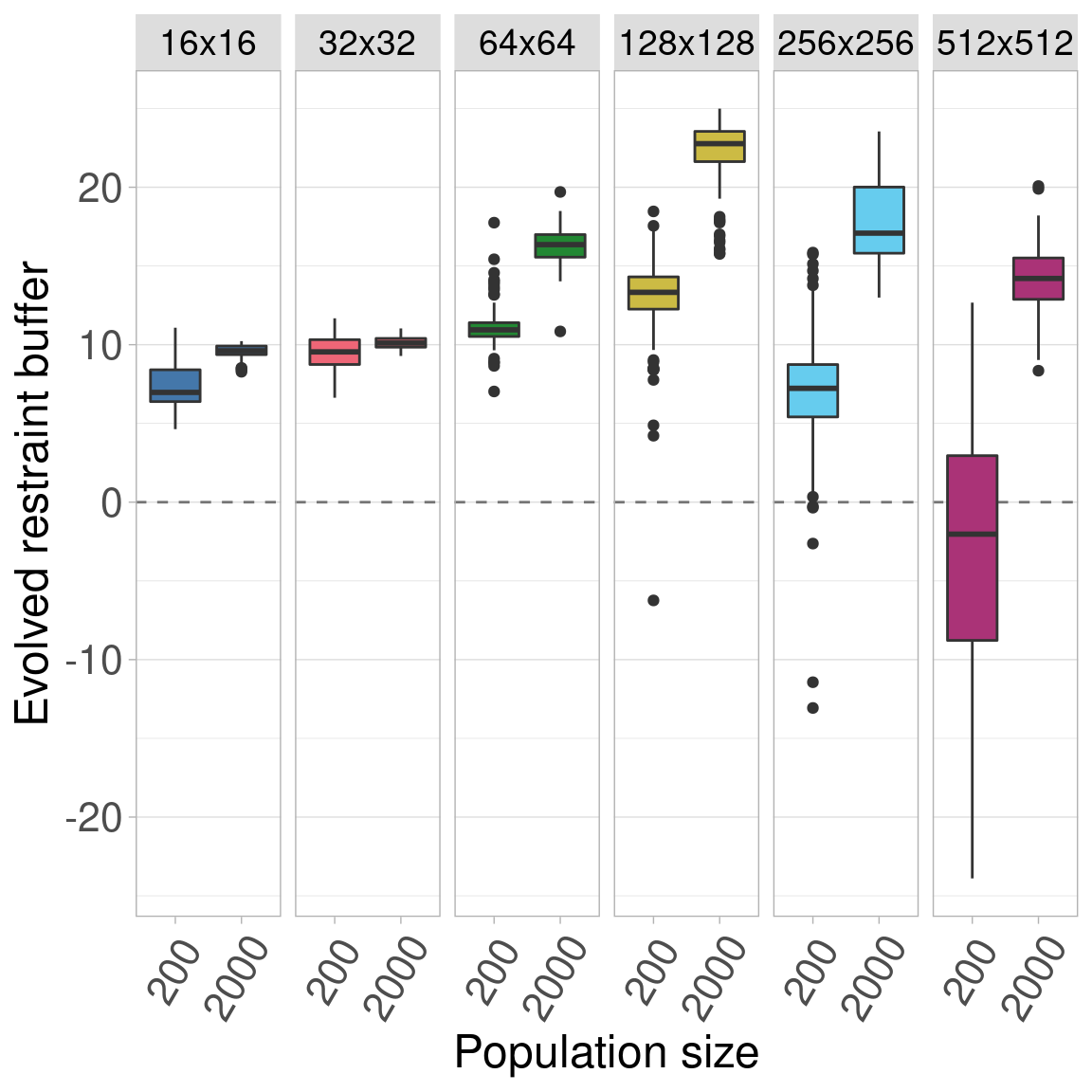
6.3 Plot

Here we plot all the data. The figure is split into 6 subplots, each showing a different organism size. Inside each subplot, population size is shown on the x-axis.

6.4 Statistics

The plot shows that increasing population size increases the evolved restraint buffer at organism sizes. Further, we see that the same general trend holds at both population sizes, that evolved restraint peaks at size 128x128.

Finally, we treat each organism size as a group and conduct a Wilcoxon Rank-Sum test between the population sizes.

##   org_size      p_value      W less_0.01
## 1       16 3.921812e-19 1341.0      TRUE
## 2       32 8.416553e-06 3176.5      TRUE
## 3       64 4.238745e-32  173.0      TRUE
## 4      128 1.013881e-33   46.0      TRUE
## 5      256 2.781080e-33   80.0      TRUE
## 6      512 4.954199e-34   22.0      TRUE